International Economics Zusammenfassung#
Definitions#
Global Trade: Sum of trade activities both within and between countries
Types of Trade:
intraregional Trade |
interregional Trade |
|---|---|
between members of economic integration space (EU, USA, country) |
between different economic spaces |
Foreign Trade: trade relations across borders
Foreign Trade Theory: explanation of occurence / impacts of foreign trade
Reasons for trade:
cost benefits
expansion of range
More availibility of goods
Gravity Model#
Amount of Trade between two countries
other Factors
Geography
cultural affinity
borders
multinational corp
Ricardo Model#
Assumptions#
one factor: labor
differing productivity across countries
supply = constant
two goods (e.g cheese and wine)
wage = price of output
Definitions#
amount of labor to produce a good: \(a_{LGood}\)
wage = \(\frac{ P_C }{a_{LC}}\)
Production Possibility Frontier = line
maximum amount of goods, producible by fixed input of factors
\(a_{LC}Q_C + a_{LW}Q_W\)
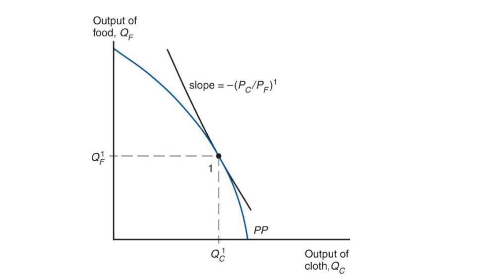
opportunity costs: \(\frac{ a_{LC} }{a_{LW}}\) = O.C of cheese
relative price: \(\frac{ P_C }{P_W}\) of cheese
Trade#
absolute advantage: country produces good with lower factor inputs
comparative advantage: country produces good with lower opportunity cost
Trade = possible when country has comp. advantage, not just absolute advantage!
O.C and Relative prices |
who produces cheese? |
|---|---|
\(\frac{ P_C }{P_W} < \frac{ a_{LC} }{a_{LW}}< \frac{ a_{LC}^* }{a_{LW}}^*\) |
Nobody |
\(\frac{ a_{LC} }{a_{LW}} \le \frac{ P_C }{P_W}< \frac{ a_{LC}^* }{a_{LW}}^*\) |
Home Country |
\(\frac{ a_{LC} }{a_{LW}}\le \frac{ P_C }{P_W}= \frac{ a_{LC}^* }{a_{LW}}^*\) |
Home Country + partly foreign country |
\(\frac{ a_{LC} }{a_{LW}}< \frac{ a_{LC}^* }{a_{LW}}^* < \frac{ P_C }{P_W}\) |
both countries completely |
Results of Trade#
Misconception |
Reality (in this Model) |
|---|---|
Trade only good for productive countries |
unproductive countries = lower wage = advantage |
Trade exploits less productive countries |
better than without, cheaper goods |
trade only good for low wage countries, not high wage |
increase wage in efficient industry in high wage country |
Specific Factors Model#
Assumptions#
3 factors (land, capital, labor)
labor = mobile
capital / land = specific to good
two goods / industries
Food = labor + land
Cloth = labor + capital
perfect competition + full employment
countries differ by many things (productivity, endowments etc.)
Definitions#
PPF = curve
diminishing returns when concentration in one industry
Marginal Product of Labor \(MPL\) = diminishing
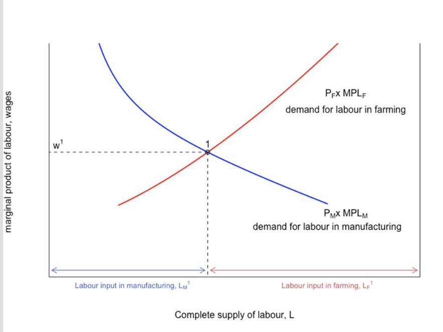
Marginal value = wage = \(P_F \times MPL_F\)
PPF |
Allocation of Labor |
|---|---|
|
|
Trade#
Amount of Goods traded depends on relative Supply supplied: \(RS = \frac{ Q_C * Q_C^* }{Q_F* Q_F^*}\)
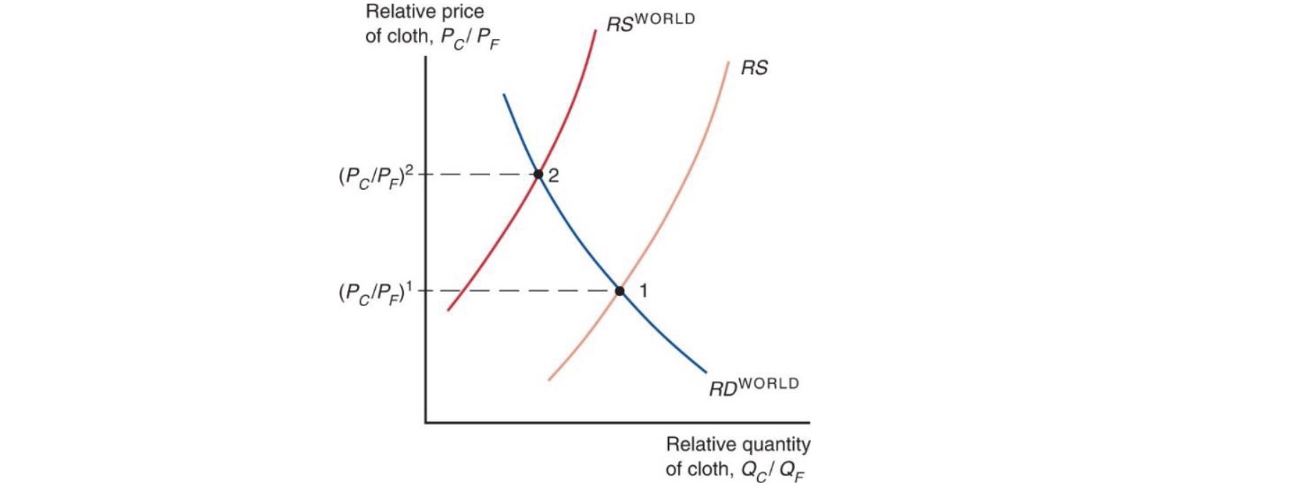
Situations:
relative quantities |
Result |
|---|---|
\(RS_{home} < RS_{world}\) |
\(\implies P \uparrow, Q \downarrow\) |
\(RS_{home} > RS_{world}\) |
\(\implies P \downarrow, Q\uparrow\) |
Results of Trade#
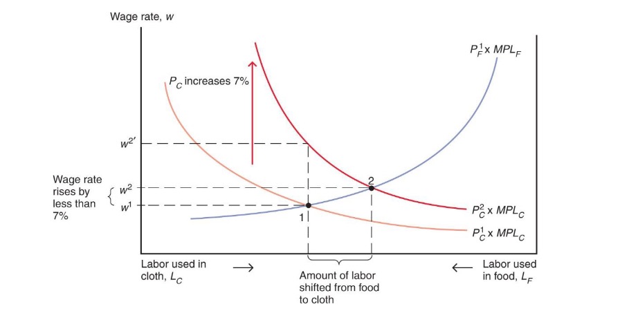
Example: Price rises of Cloth
Output rises
capital owners profit
labor shifts from food to cloth
wage does not rise as much as price (%)
worker profit = depends on preferences
Results depend on if sector is export or import sector
Budget Constraint above PPF = achievable
Heckscher-Ohlin Model#
Assumptions#
two goods (food and clothing)
two factors = mixed across goods
free capital / labor mobility
countries only differ by endowments
Definitions#
Production of Good depends on Production Function \(Q_C = f(K,L)\)
Capital-intensive industry (cloth): \(\frac{ a_{KC} }{a_{LC}} > \frac{ a_{KF} }{a_{LF}}\)
PPF
\(V = P_C*Q_C+P_F*Q_F\)
\(K \ge a_{LF} Q_{LF}+a_{LC}Q_{LC}\) (Capital allocation across sectors)
smooth curve!
Producers: choose factors based on wage and r (interest)
higher wage = offset by more capital input
Trade#
Countries produce goods intensive with their abundant factor
e.g USA = capital abundant = produce computer
Bangladesh = labor abundant = produce clothes
moves Relative Supply (like in Specific Factor)
same preferences = same consumption after trade
Autarky |
Trade |
|---|---|
|
|
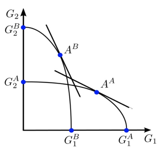
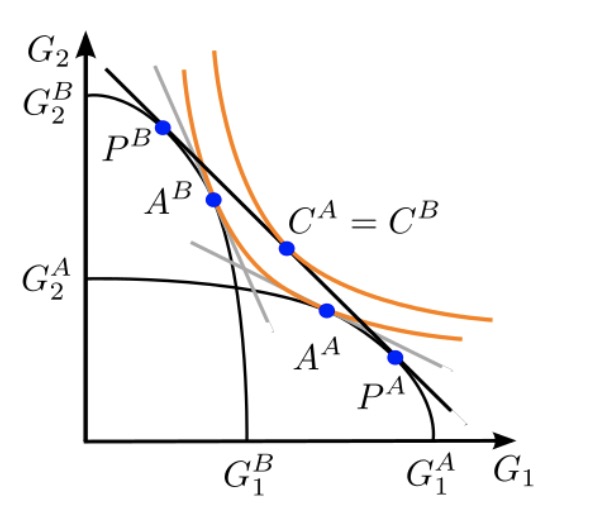
shows two different countries (A & B) with factors (\(G_1\) & \(G_2\))
Results of Trade#
prices converge
countries specialise
Owners of abundant factor profit (capitalists in US, workers in Bangladesh)
other factors = less produced = diminishing returns
redistribution across owners, not industries!
Standard Model#
generalizes all models (with others as special cases)
Assumptions#
two goods
each country individual PFF, differences between
factor endowment
technology / productivity
Definitions#
PFF = smooth curve
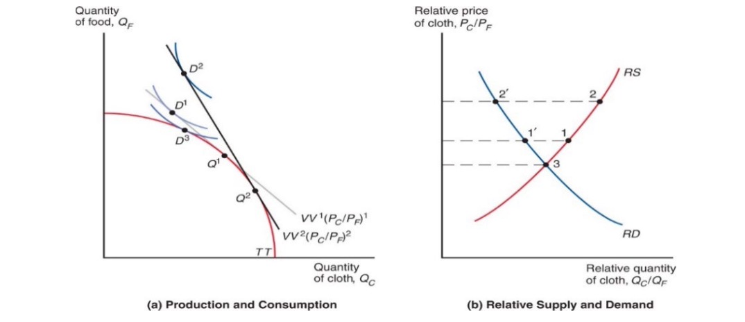
production depends on relative price \(\frac{ P_F }{P_C}\) and
Indifference Curve of Consumers
different isovalue lines and PPF
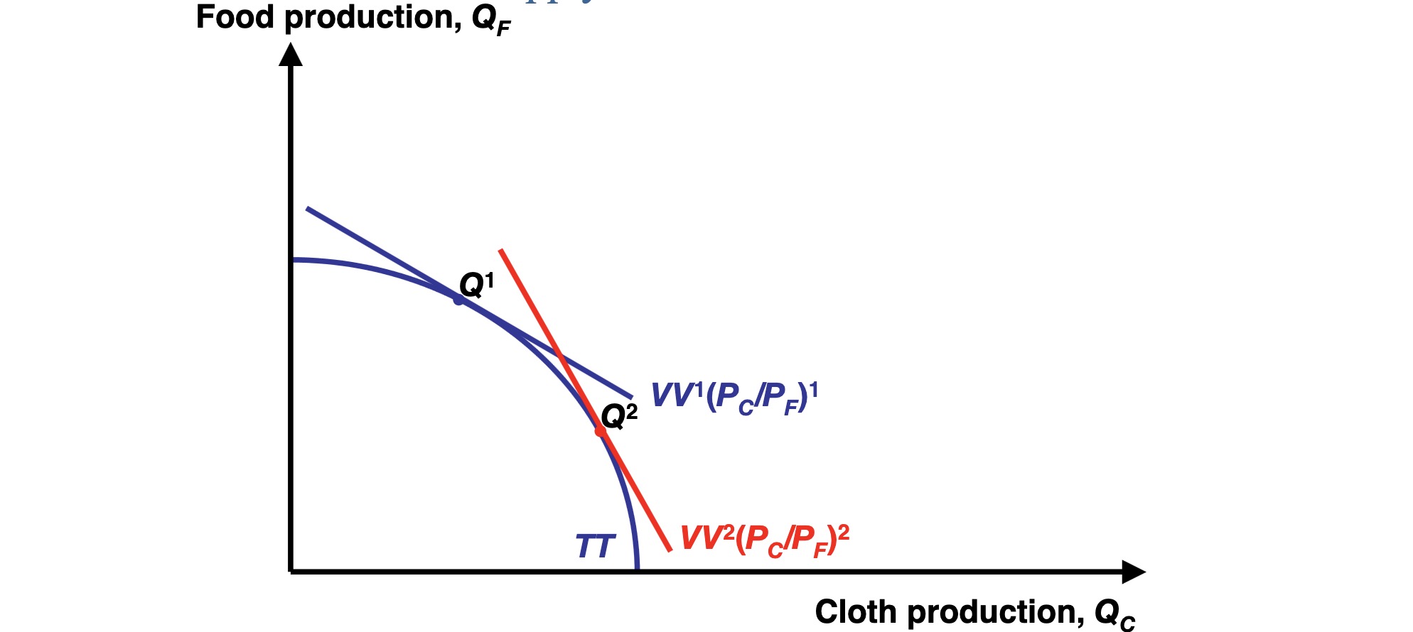
Trade#
depends on relative prices
and Terms of Trade \(= \frac{ Price_{exports} }{Price_{imports}}\)
rise = good for welfare of country
Allows higher IDK than without
Results of Trade#
grows economy (mostly biased growth)
depends if growth in export or import sector
import biased growth = higher ToT = welfare gain
export biased growth = lower ToT = welfare loss
Model Comparison#
Model |
Assumptions |
differences between countries |
Time perspective |
winners of trade |
|---|---|---|---|---|
Ricardo |
one factor, 2 goods |
labor productivity |
short run |
everybody |
Specific Factor |
3 factor, 2 goods |
Productivity / factors |
medium run |
export industries and their factors |
Heckscher Ohlin |
2 factor, 2 goods |
Endowment of Factors |
long run |
owners of abundant factors |
Standard |
2 factor, 2 goods |
Everything |
Depends |
3 models = 3 time frames of factor mobility
ricardo = immobile = short run
specific factor = partly mobile = medium run
heckscher = very mobile = long run
shock is dynamic over time frame
Theorems#
all in the Heckscher Ohlin Model
Heckscher-Ohlin Theorem: countries specialize in goods that use its abundant factor intensively
e.g Bangladesh labor-abundant = clothes production
Stolper-Samuelson Theorem: Rise in relative price of good => higher return to factor used intensively & lower returns for factors of other good
e.g higher price for clothes => higher wages for clothes workers & lower returns for land owners in food production
Rybczynski-Theorem: if prices constant and amount of one factor rises => Quantity of good using factor intensively increases & other goods quantity decreases
e.g population rise in Bangladesh => more clothes produced & even less food production
Trade Policy Instruments#
Policy |
Producer Surplus |
Consumer Surplus |
Government revenue |
national Welfare |
|---|---|---|---|---|
Tariff |
+ (increase) |
– (decrease) |
+ |
~ (Depends on country size) |
Export Subsidy |
+ |
– |
– |
– |
Import Quote |
+ |
– |
= |
~ |
Voluntary Export Restraint |
+ |
– |
= |
– |
Tariff#
Tariff: tax imposed by government on imports, either per unit (specific) or as % of value (ad valorem)
similar to transportation cost
higher price at home
lowers world market price (if country big enough)
decreases quantity traded
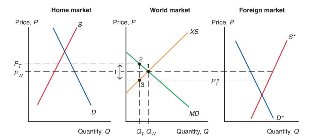
producers profit, government gains revenue, consumers have to pay higher prices
Export Subsidy#
Export Subsidy: policy to encourage export of goods and discourage sale of goods on the domestic market through direct payments
lowers price in importing countries
higher price for home consumers
Import Quota#
Import Quota: Restriction of Quantity of Good that may be imported
no government revenue
quota rents to license holders
Voluntary Export Restriction#
Voluntary Export Restraint (VER): quota imposed by exporting country on its exporting industry
due to pressure by Importing Country
Example: Japanese Cars in US Market
Price rose of japanese fuel efficient cars
rent to japanese firms
Local Content Requirement#
Local Content Requirement: regulation, that fraction of end product domestically produced
no revenues
home producers of inputs like import quota
home producers of outputs not as strict
price diff average between no quota and import quota
Political Economy of Trade#
International Trade & Globalisation = highly debated topic
Case for Protection#
Presence of imperfect markets
No prefect competition
market distortions
Examples:
tariff on foreign monopoly firm = shift profit to domestic
subsidy on domestic firm = compete against oligopolies
Brender Spencer Analysis
capture world market = higher profit than subsidy costs
Example: Airbus - Boeing
pollution = negative externality
tariff = shift to less polluting domestic industry
less world pollution overall
Case against Protection#
Retaliation
possibility of retaliation of other countries
less welfare overall
Superior Policies to raise efficiency
if goal is to stop unemployment
use fiscal policy e.g than trade policy
Trade policy = Second Best Option
Information Deficiencies
perfect tariff rate = difficult to set
unintended consequences in other industries
Lobbying / Rent Seeking
concentrated interest groups = more power than less concentrated consumers
captured by special interests