21.06.2023 Inflation and monetary policy#
Inflation and Philipps Curve#
Inflation: Increase in general price level, measured by CPI
Real interest Rate \(r = i - \pi^e_{t+1}\) (Fisher Equation)
also measured with differnce between inflation indexed bonds and market bonds
rational expectations formulation:
no systematic forecast errors
use all relevant info (esp. expert forecasts)
problem: incomplete models and experts
Problems
volatile / high = detrimental
investment unsafe
income declines
Benefits
effective monetary policy (no deflation)
redistribution (creditor to debtor)
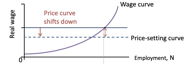
Wage as Inflation Driver#
also: Demand Pull Inflation
Owners Power rises (e.g lower comp.)
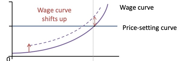
employees power rises (e.g. more people join union)
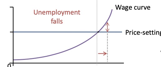
Unempl. falls
Situation |
Graphic |
|---|---|
Owners Power rises (e.g lower comp.) |
|
employees power rises (e.g. more people join union) |
|
less unemployment (more power) |
|
Philipps Curve: Unemployment and Inflation
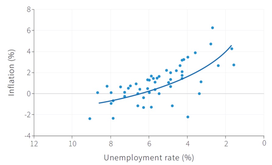
=> curve can shift over time (stagflation)
other reasons: Capacity Constraints (in the short run)
AD, Unemployment and Inflation#
Labor Equilibrium shocks#
Bargaining Gap: Difference between real wage with highest incentive and real wage with highest profit
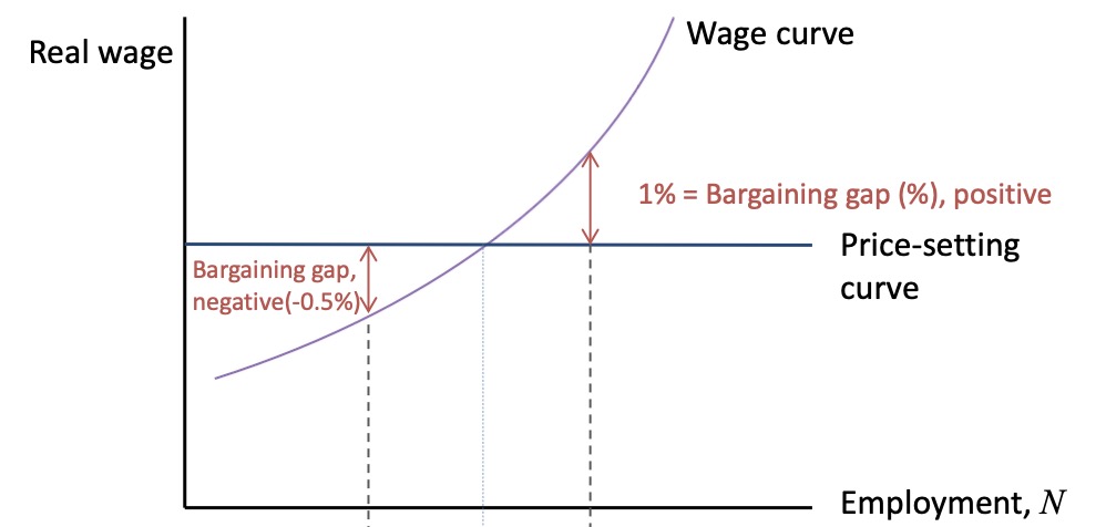
Calculated:
translates to
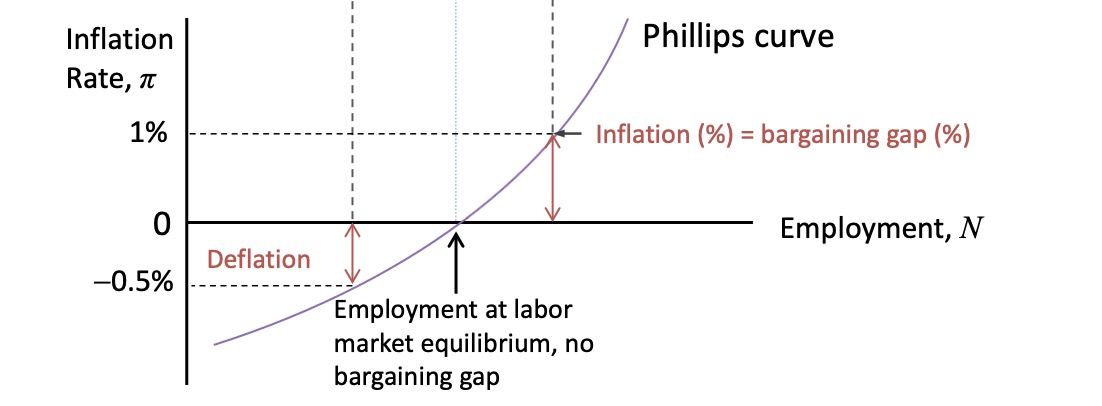
Medium-Run:
Boom (higher AD)
less unempl.
positive bargaining gap
positive wage-price spiral
Inflation
Recession (lower AD): vice versa
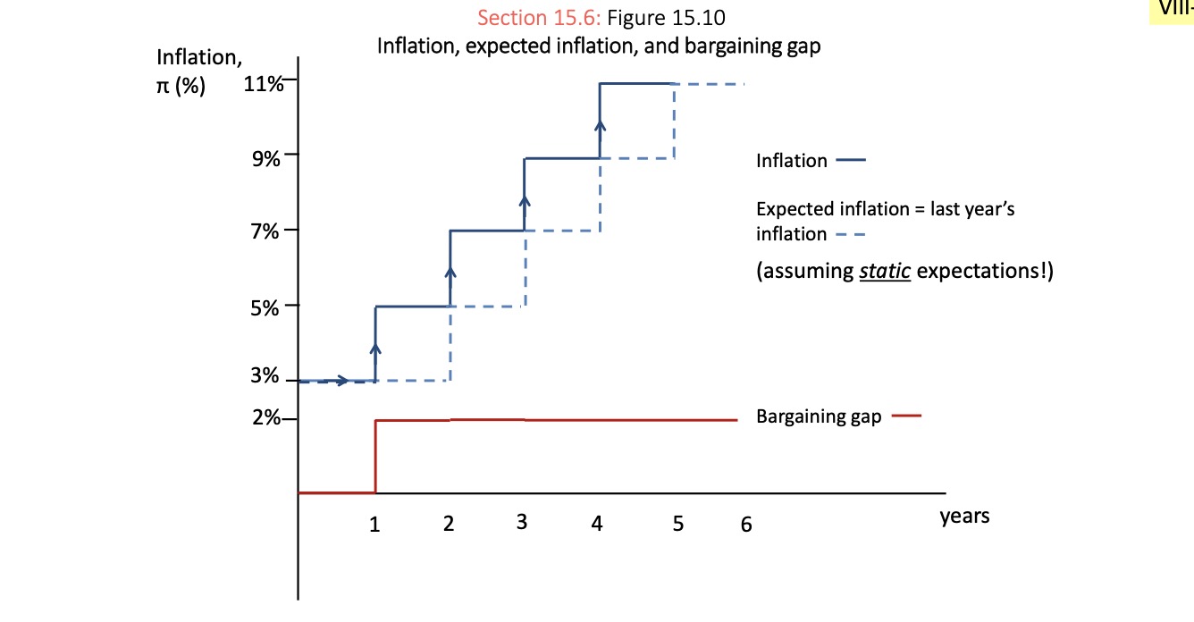
in Boom:
workers want real wage rise and inflation combat rise
these rises oush next years inflation etc…
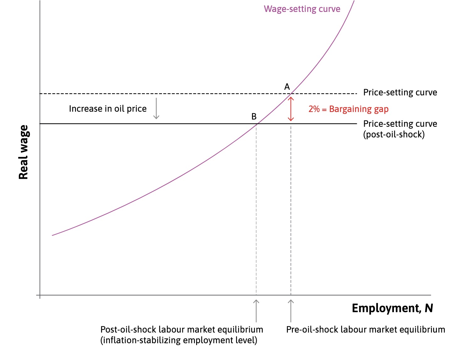
Supply Shocks#
Price Shocks to the material supply:
Firms rise prices to protect profits
workers lose real purchasing power
=> bargaining gap
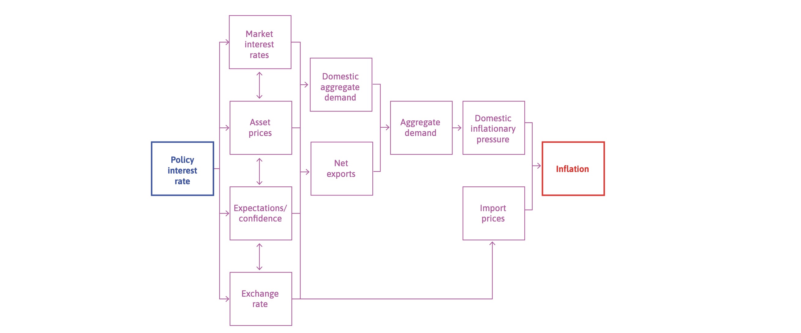
Monetary Policy#
Transmission channels on Inflation
market interest rates
value of assets
expectations
exchange rate
Limitations:
zero lower bound
long maturities
=> alternative Quantitative Easing
Interest rate Yield curve#
different interest rates depending on maturity
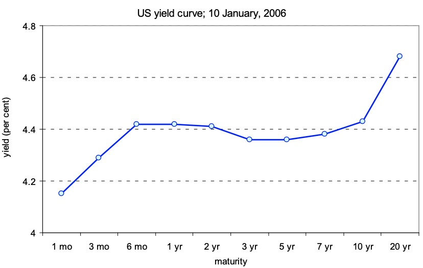
Reason: rational expectations because of higher risks for investors
=> investors arbitrage the interest differences based on the expectations for future interest rates
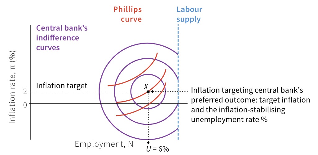
Barro-Gordon Model#
Model about Central Bank actions with inflation targeting
Loss Function of CB:
\(U / U^*\) = unemployment / target rate for unempl.
\(\pi / pi^*\) = inflation / target rate of inflation
b = vaulation of other goals beside inflation, here Unemployment
higher b = more flexible inflation target
Barro Gordon Model#
Expectations-augmented Philipps Curve:
\(U_n\) = natural rate of unemployment
when inflation differs from it, then another U possible
Optimal Point (bliss point):
\(U^* = k * U_n; 0 < k < 1\)
\(\pi^* = 0\)
Combination of L and U Formula and Bliss point
Explanation of this calcukation an graph: what if the central bank is not independent and has the will to lower unemployment? then they will create a surprise inflation:
Starting in Point A: expecations = 0, full power to CB
Goal is Point B with lower unemployment
but Result is D, due to actors incorporating the expected inflation
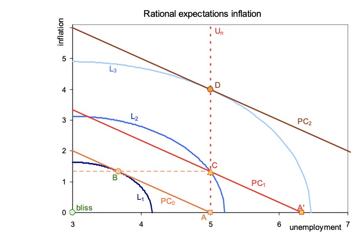
=> Credibility needed
Central bank works with expectations
higher credibility = easier policy
no expected surprise inflation
with policy rule = 2% = rational expectation
CB stays at Point A
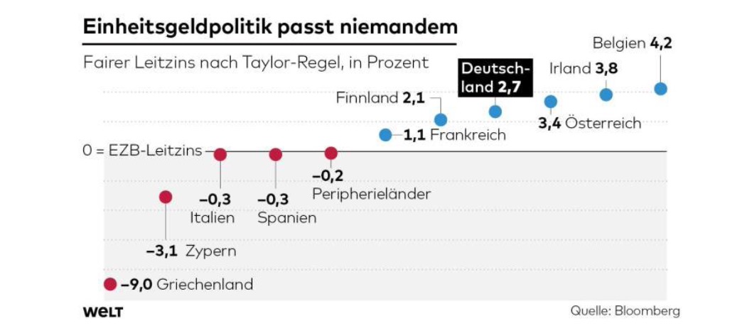
Taylor Rule#
Rule of John Taylor for central banks short term rate $\( i_t-\pi_t = r+a(\pi_t-\pi^*)+\beta x_t \\ with \ x=\frac{ Y -\bar{Y}}{\bar{Y}} = output \ gap \)$ CB should adjust short term rate based on heating of the economy
in Euroarea: not possible, due to unified monetary policy
and output gap estimation difficult
From the typical euro critics at Axel-Springer:
better version of this: Orphanides Rule