Macro 2 Summary

Table of Contents:

• Labour Market

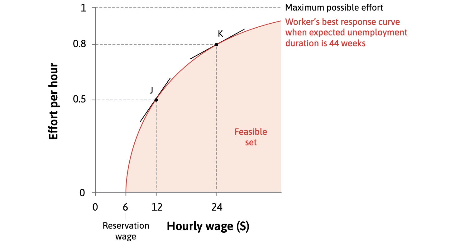
  • Wage and Effort

  • Wage Setting

  • Prices

  • Price Setting

  • Equilibrium

• Banks

• Business Cycle

  • Definitions

  • Smooth Consumption

  • Volatile Investment

  • Government Expediture

  • Stylized Facts

  • Multiplier Model

  • Influences on the Multiplier Model

  • AD and Unemployment

• Government

  • Important equations

  • Phase Lines

  • Default Risk

• Inflation

  • Philipps Curve

  • Bargaining Gap

  • Inflation and AD

  • Expectations

  • Monetary Policy

  • Preferences of CB

Labour Market

Wage and Effort

= individual worker

• wage set in contract, depends on

  • reservation wage = outside option

  • disutility of effort

  • employment rent

=> firms set wage based on effort level needed (HR Department)

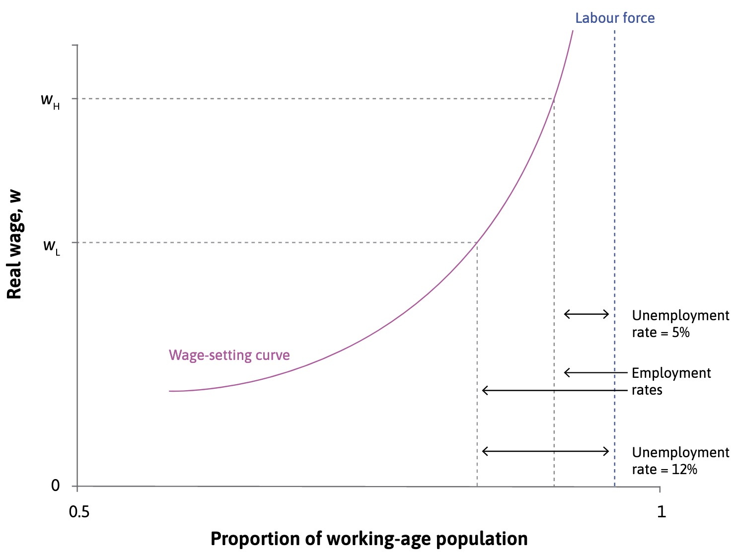
Wage Setting

= whole economy

• based on unemployment in economy

• gives general wage level (nominal)

=> higher unemployment = lower nominal wage

individual	whole economy

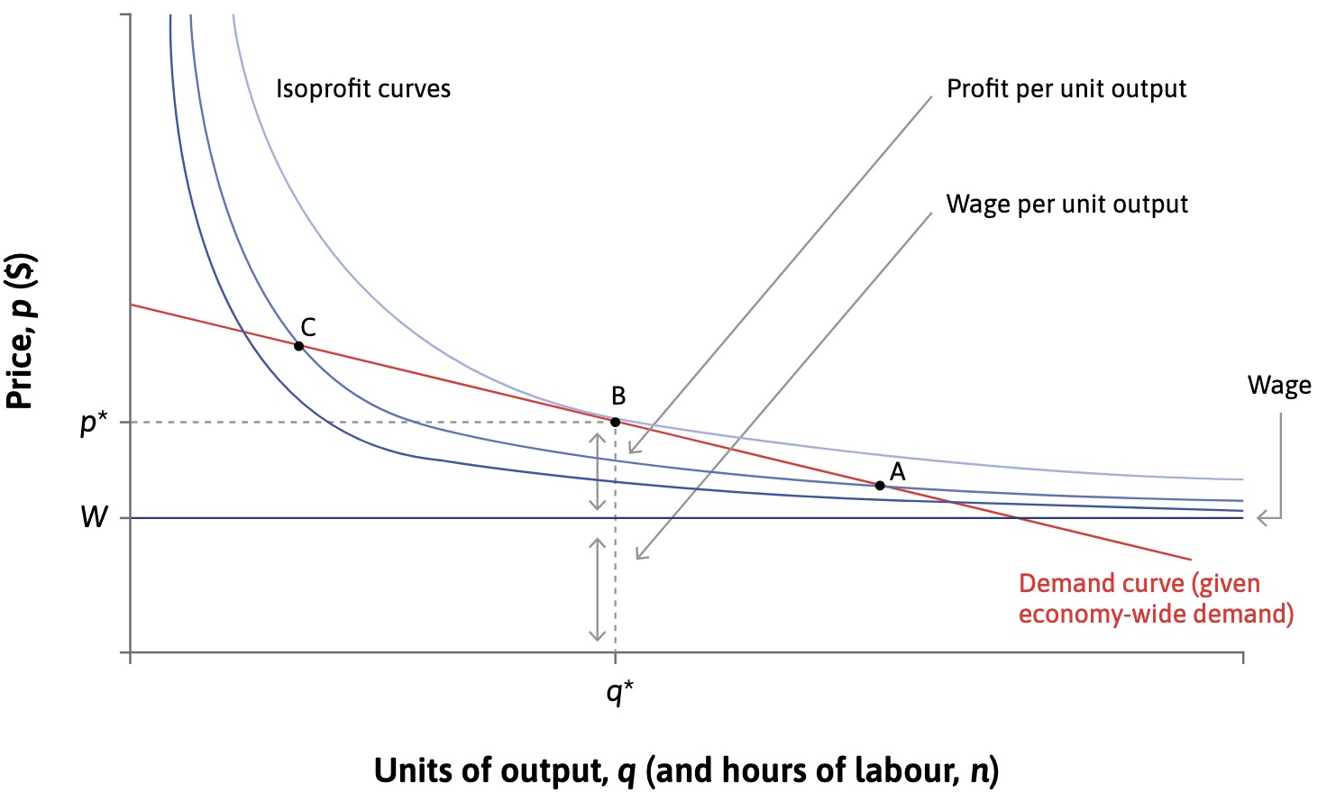
Prices

= at individual firms

Firms Decision at given Wage based on

• Demand

• Competition

• Markup needed for shareholders

=> prices / level of output and number of needed workers

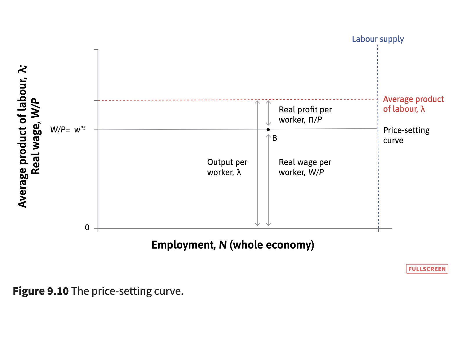
Price Setting

= whole economy

• all prices combined lead to price level

• real profit per worker (\(\Pi/P\))

• real wage per worker (\(W/P\))

=> only depends on competition

indivudual firm	whole economy

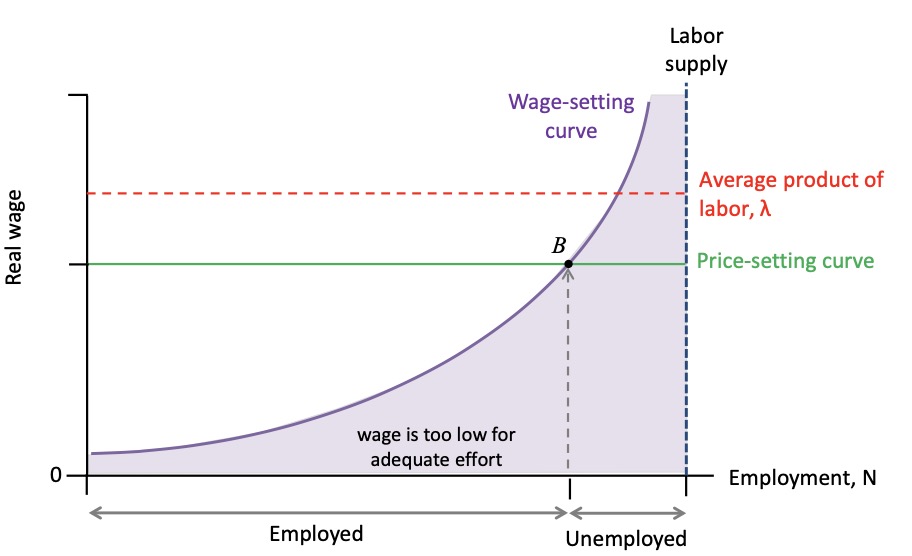
Equilibrium

• Wage Setting: Wage at given Effort

• Price Setting: Prices at given Markup

leads to

• least wage for effort

• maximum employment

• Involuntary unemployment (due to incomplete contracts!)

Model reaction to lower AD:

• higher unemployment

• lower wages along the WS-curve

• lower prices for goods

• higher demand for goods = higher labor demand

• more employment back at equilibrium

Problem: Sticky Wages! and savings

Solution: Government Intervention to expand Demand (Monetary or Fiscal)

Banks

lets just hope that banks dont play a big role in the exam…

Business Cycle

Definitions

Type of Fluctuations in capitalist economies of aggregate economic activity between contraction and expansion

Okuns Law: Connection between Cycle and Unemployment

Recession: Significant decline in economy-wide activity

GDP: Gross Domestic Product, calculated in different ways:

• Income

• Spending

• Value added in Production

Spending: \(Y = C+I+G+X-M\)

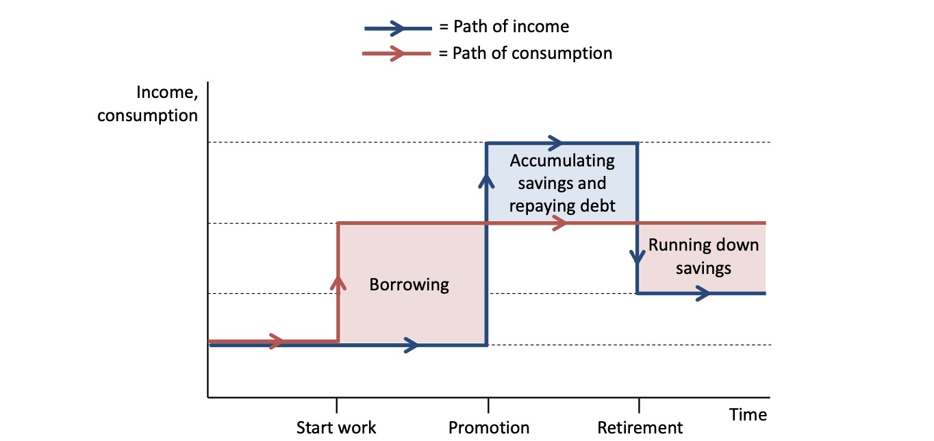
Smooth Consumption

individuals smooth consumption (to have higher quality of life)

• Borrowing from future income

• saving / repaying in high-income times

limited by:

• credit constraint

• weakness of will

• limited insurance

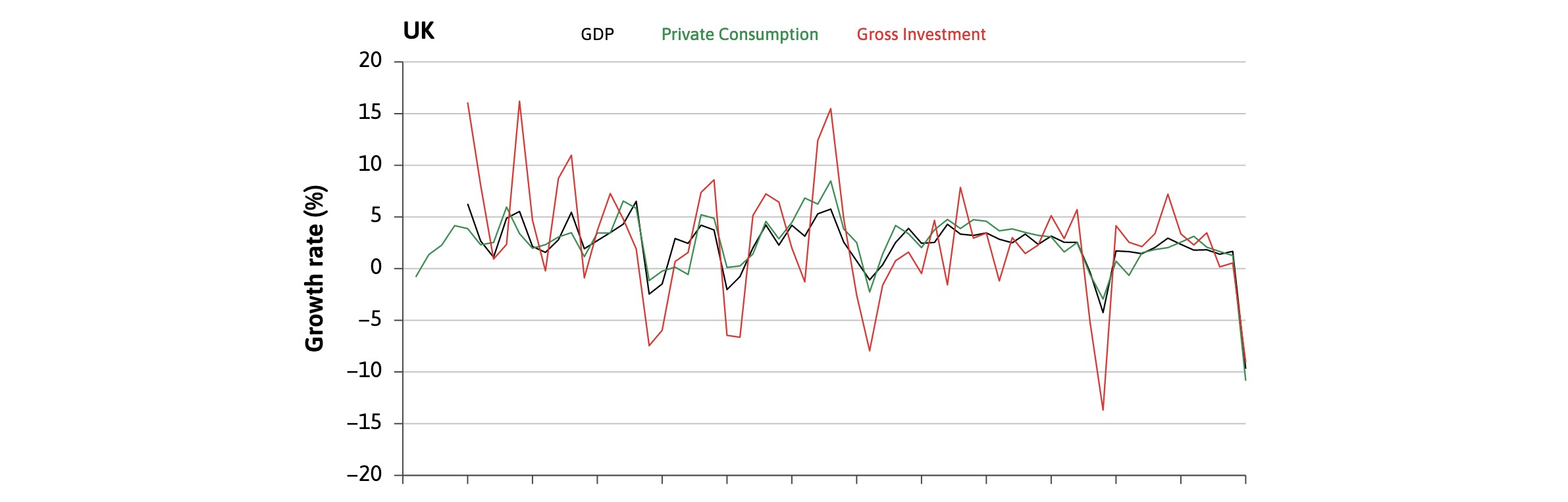
Consumption: lagging GDP, highly correlated

Volatile Investment

Investment = depends on expectations regarding BC

Contraction	Expansion

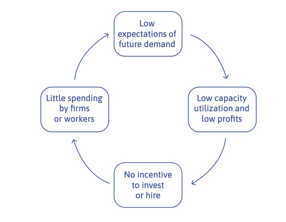
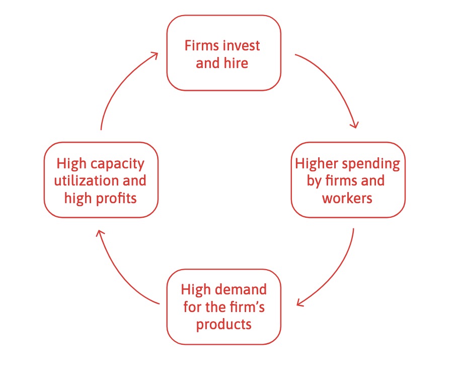
leads to self-enforcing business cycles

Investment: leading GDP, high volatility

Government Expediture

Share of Government spending on% of GDP (\(b\))

• varies across countries

• depends on taxes / other income

• finacable by debt / money print

Government Expenditure: less volatile than GDP, not dependent on expectations

Stylized Facts

Volatile	Correlation	Persistence	Leading / Lagging
Investment = more volatile than GDP	Consumption / Investment = correlated to GDP	GDP + Investment = persistent	Investment = leading GDP
Inflation = less volatile	Infaltion | GDP = no strong correlation	G Exp + Employment = very persistent	Employment = lagging GDP

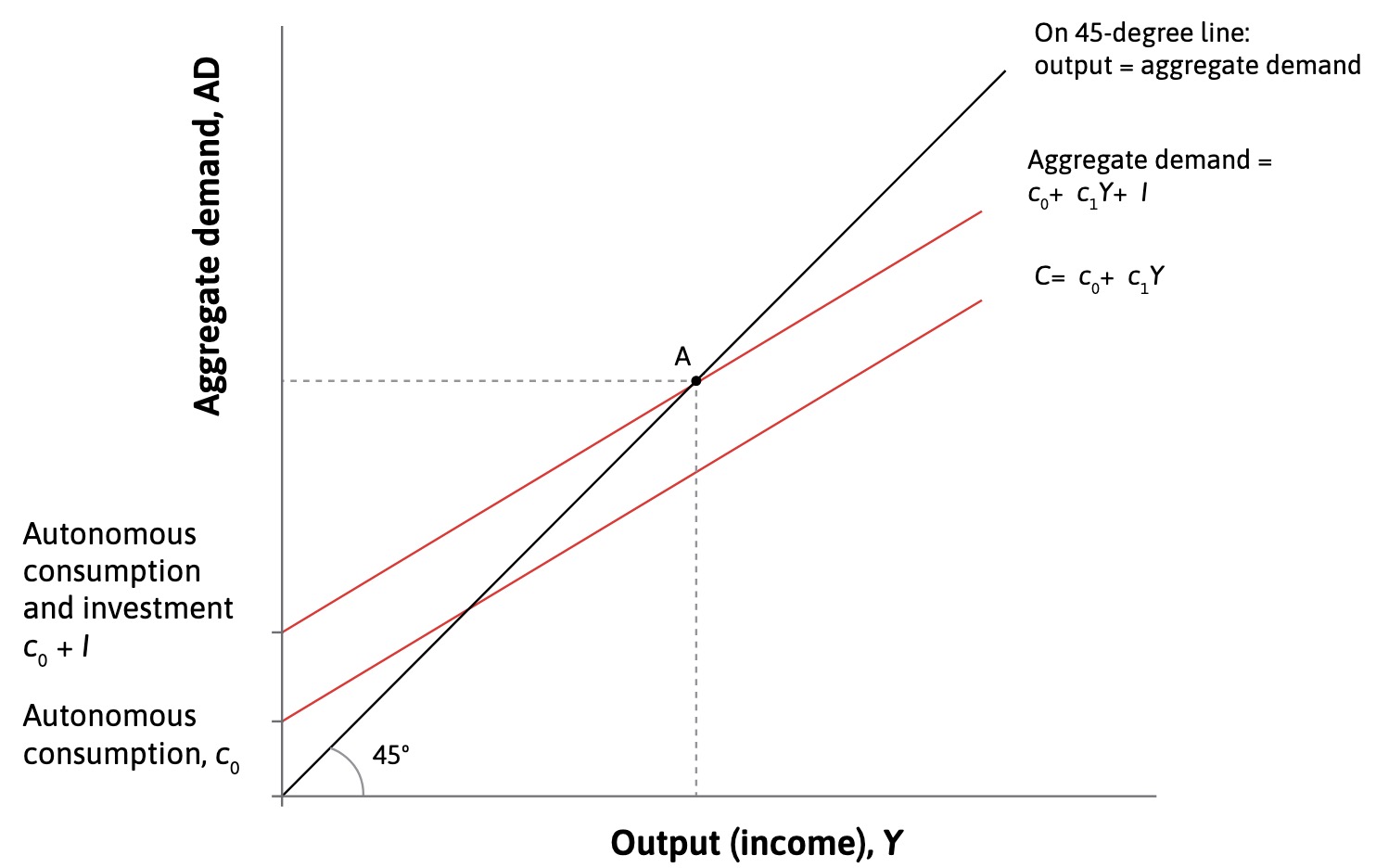
Multiplier Model

Consumption Function:

• autonomous consumption (from smoothing): \(c_0\)

• income dependent consumption: \(c_1*Y\)

  • based on marginal propensity to consume

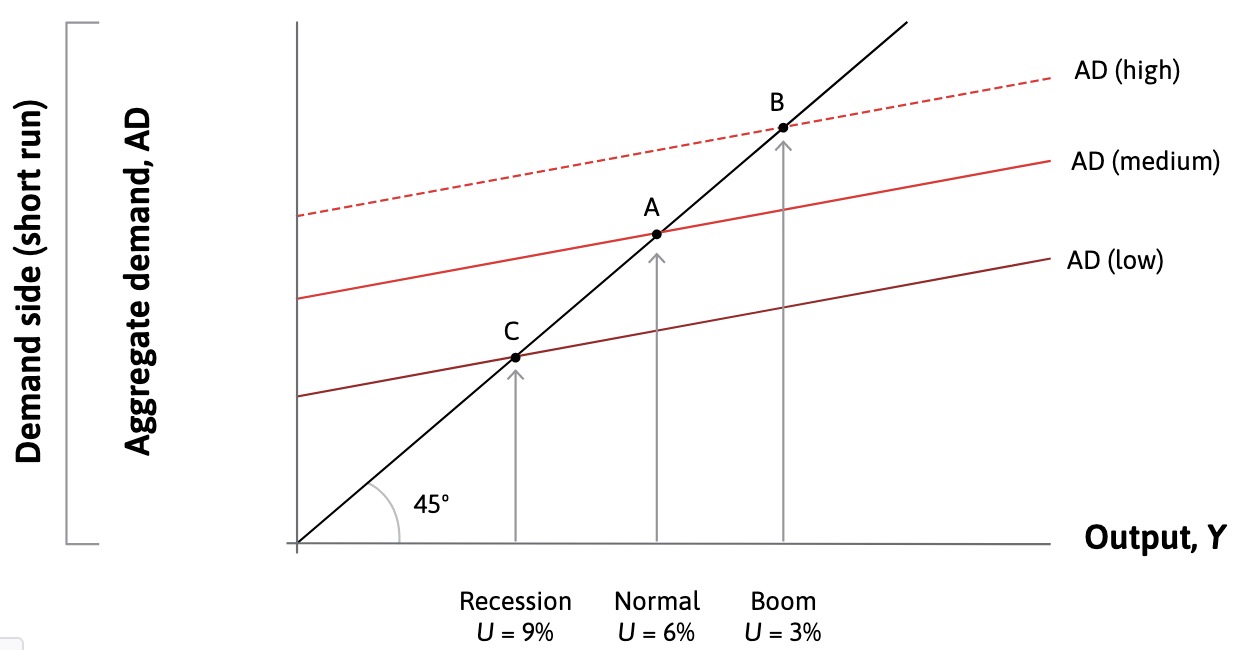
• 45° Line = Aggregate Demand = Aggregate Supply

  • Everything needed is supplied (at less than full capacity)

Change in Output / Income: never relevant, moves along the line

Change in AD: relevant, because it moves the line (e.g \(I, G, c_0\) change)

• exampe: higher Investment

• moves Consumption Line upwards

• multiplied by after round effects

Multiplier: \(k = \frac{ 1 }{1-c_1}\)

Influences on the Multiplier Model

Fiscal Policy = dampen Fluctuations in AD

Multiplier influenced by

• Exports / Imports = make Stimulus more difficult

• high credit constrained = more effective multiplier

• Capacity of Economy

AD and Unemployment

Connection of both Models

• Supply Side: Labor Market Model

• Demand Side: Multiplier Model

Assumption: \(N = Y\)

Government

Role = Fiscal Policy in Crisis, when k > 1 (output gap)

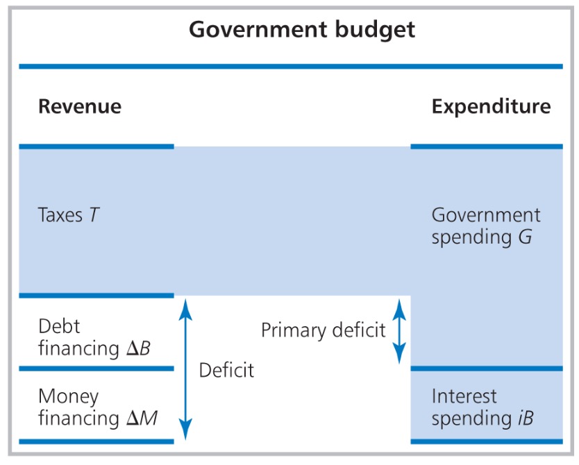
• Budget Deficit: \(\Delta B = G+iB-T\)

• Primary Deficit: \(G-T\)

• Budget Constraint: \(T + \Delta B = G+iB\)

Important equations

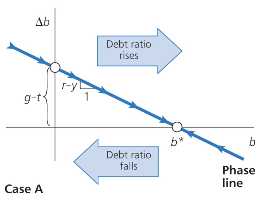
• \(\Delta b = g-t+(r-y)b\) : debt ratio dynamics

• \(b^* = \frac{ g-t }{y-r}\) : equilibrium debt ratio

  • \(b^* < 0\) = creditor

  • \(b^* > 0\) = debtor (should be at least)

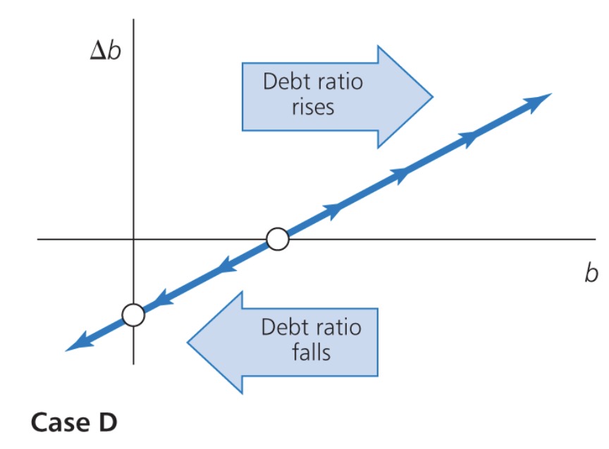
Phase Lines

Stability of Debt

• if \(r-y < 0\) (growth higher than interest) = repayment always possible

• if \(r-y > 0\) (high interest rate) = debt spirals out of hand

stable creditor	unstable creditor

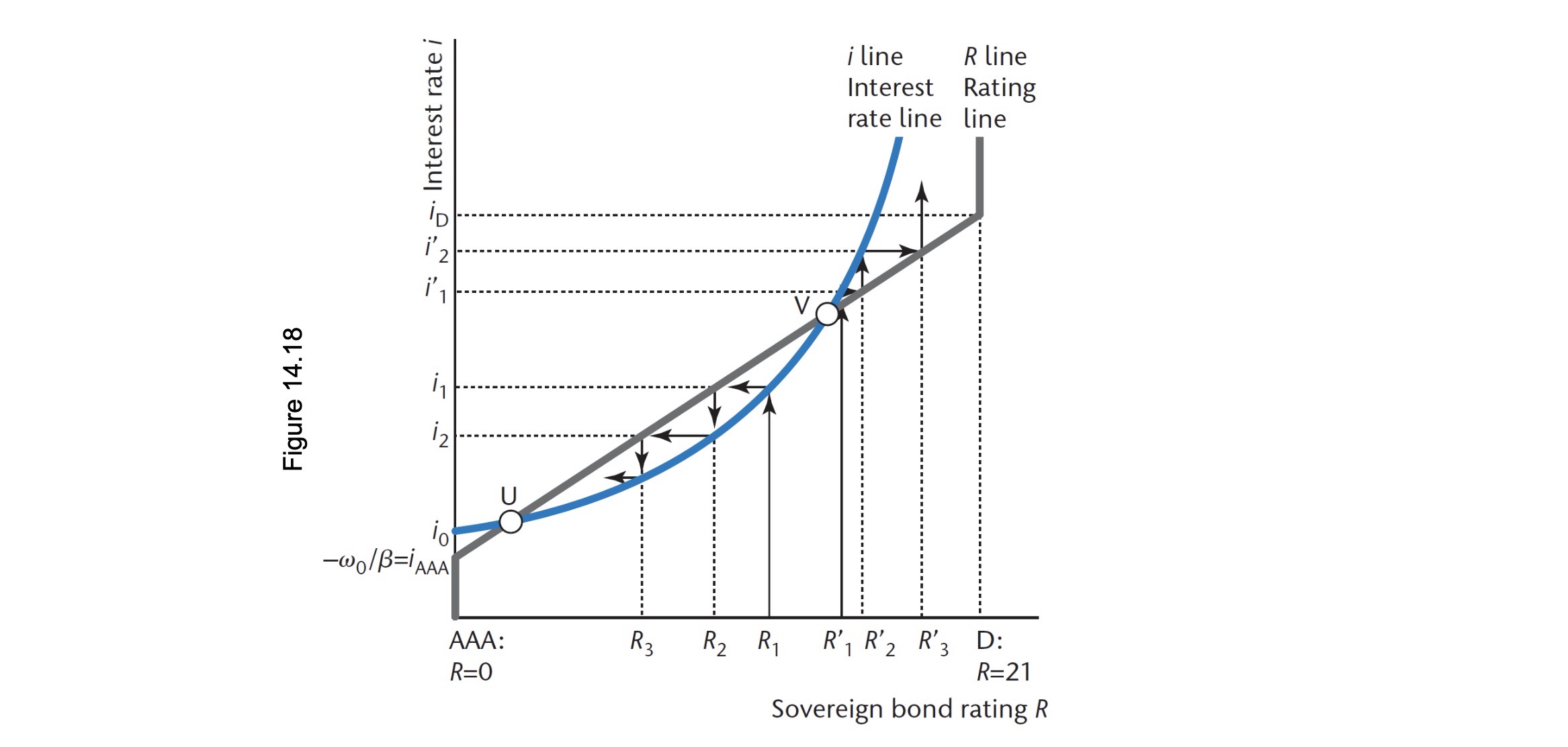
Default Risk

• default probability: \(\omega\) (determined by credit agency)

• \(i_0\) = riskless asset

Government Interest Rate:

\[ i = \frac{ i_0+\omega }{1- \omega} \]

Default Risk: \(\omega = \omega_0 + \beta i\) (Debt ratio and interst are in calculation)

Risk of Spirals: interest rate \(\uparrow\) = debt burden \(\uparrow\) = risk \(\uparrow\) = interest rate \(\uparrow\)

Bond Rating (R) and interest rate:

Inflation

Inflation: increase in general price level

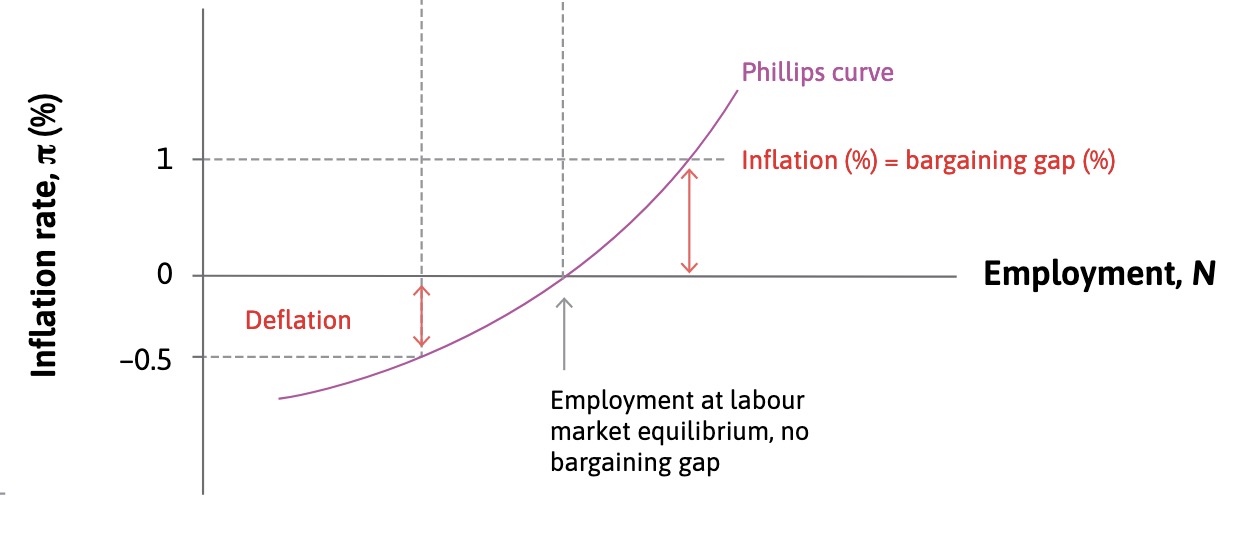
Philipps Curve

Correlation between Unemployment and Inflation (inverse relationship)

Higher unemployment = lower wages = lower prices = lower inflation

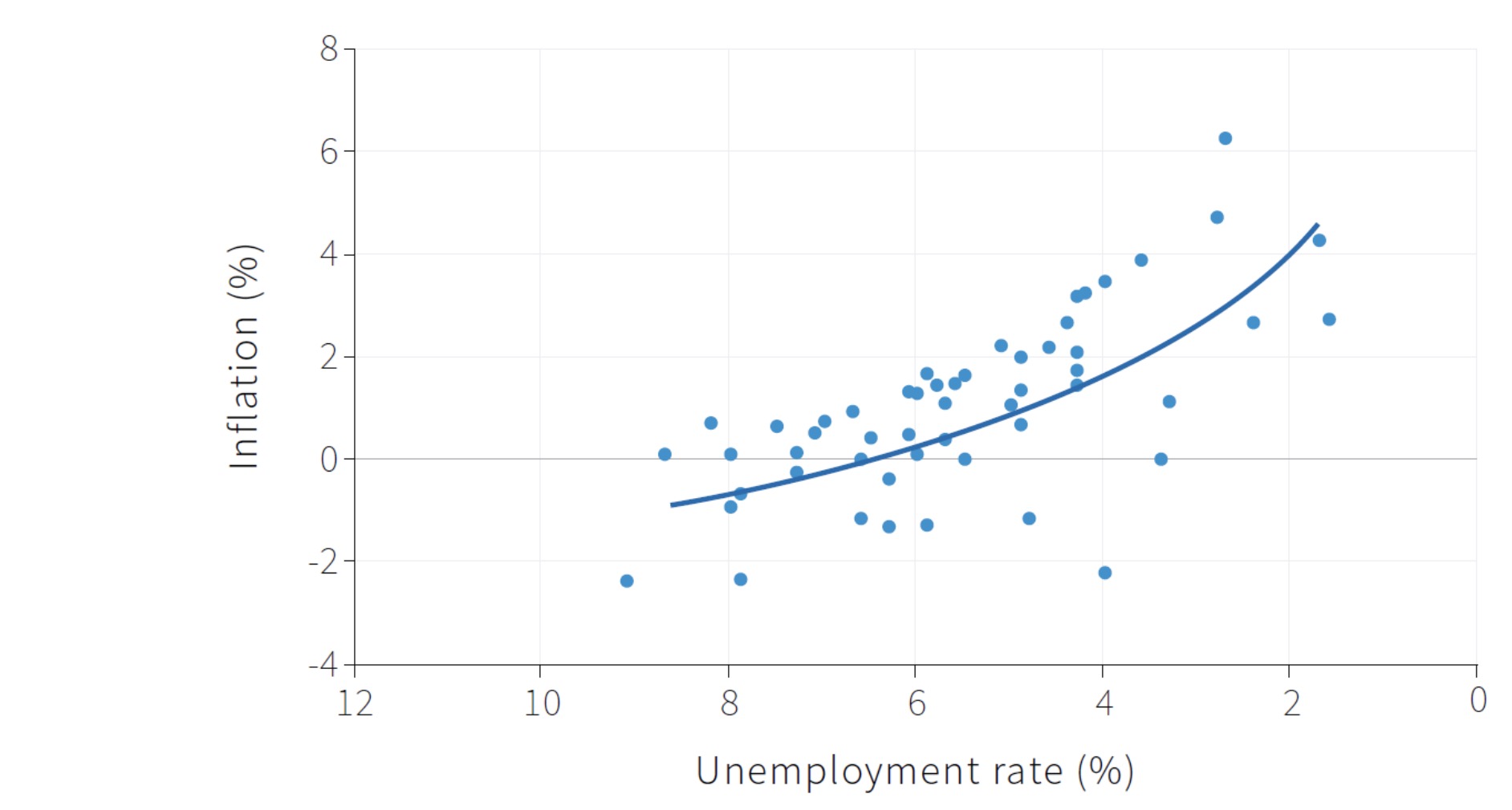
=> the philipp curve shifts with expectations of inflation! (staglfation)

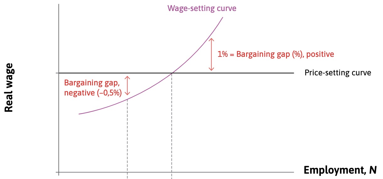
Bargaining Gap

Difference between:

• Wage firms want to offer for optimal effort (Wage Curve)

• Wage for optimal markup (Price Curve)

=> inconsistent claims in output

possible Reasons:

• higher firmpower = higher markup = lower PS

• higher union power = higher wages = higher WS

• more employment = WS \(\to\)

Inflation and AD

Combination of

• short run model (Multiplier Models)

• and medium run (efficiency wage model)

Effect of Boom:

• lower unemplyoment

• WS curve to the right

• higher wages + bargaining gap

• higher prices

• Wage price Spiral

AD	Wage	Phillips

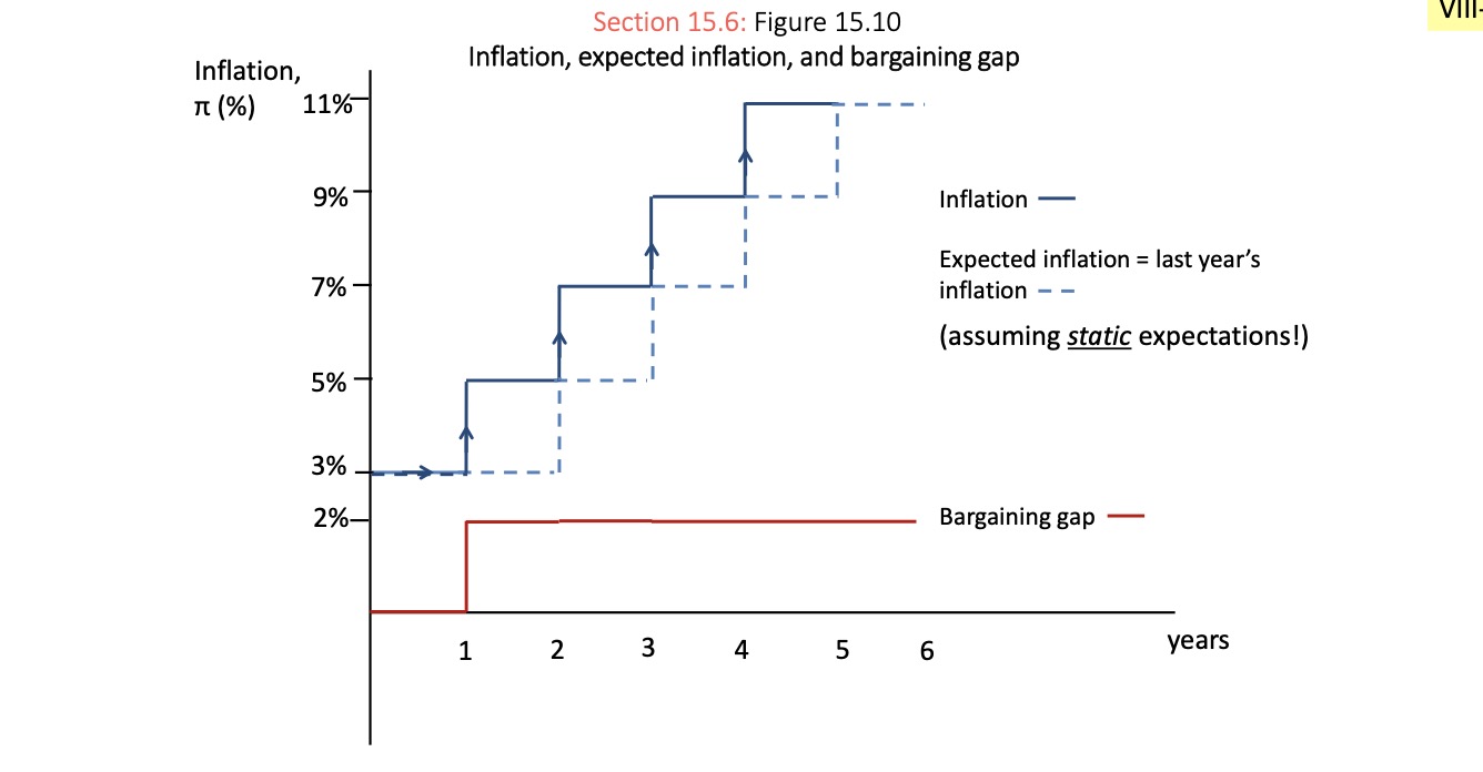
Expectations

Friedman: Expectations are integrated into inflation => no long term suprise infaltion possible

Phillips Curve Tradeoff not possible!

Situation:

• normal inflation = 3%, Bargaining Gap = 2%

• workers demand wage rise of 5%

• but inflation next year = 5% => demand 7%

depends on static expectaions \(\pi^e = \pi_{t-1}\)

Spiral of Inflation:

Monetary Policy

Tools:

• interest rate, influences

  • market interest rates (investments)

  • asset values

  • expectations

  • exchange rate

• Quantiative Easing

Assumptions of effective MP:

• independence

• above zero bound

• flexible exchange rate

• own currency

Problems:

• Trust needed

• Fiscal Policy = can have opposing goals

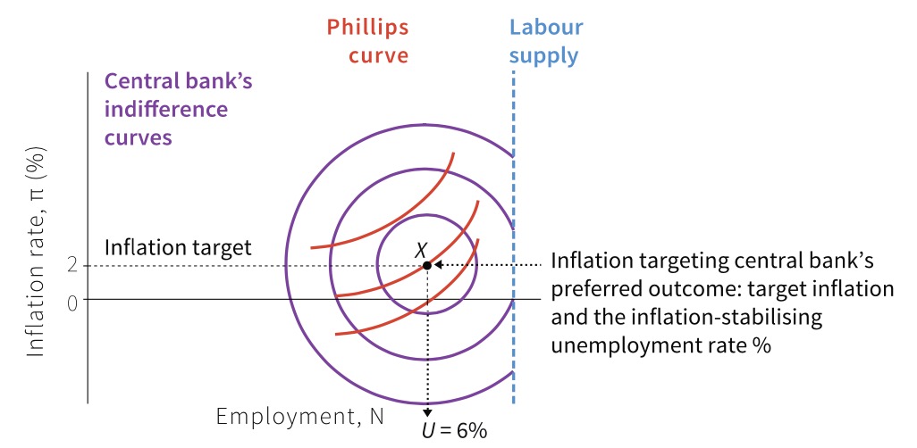
Preferences of CB

Loss Function: \(L = b(U-U^*)^2+(\pi-\pi^*)^2\)

Optimisation: \(U = U_n - a (\pi-\pi^e)\) (Phillips Curve with Expectations)

=> Surprise inflation = incorporated = not worth it

defines rule-based inflation targeting: