11.04.2024 Simple Regression

Basics

Basic Structure:

\[ y = \beta_0 + \beta_1 x + u \]

only one explanatory variable

• y = dependent / explained / regressand

• x = independent / explanatory / regressor

• u = unobserved

Functional relationship:

• x ~ y (linear)

• \(\beta_1\) = slope

• \(\beta_0\)​ = constant / intercept

• u = unobserved factors

Note: linear is not always realistic assumption!

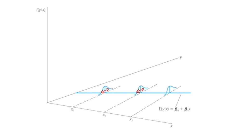
Assumptions:

1. \(E(u) = 0\) : avg. unobserved is zero

2. \(E(u | x) = u\): conditional average is independent

   • avg. of u does not depend on x!

3. \(E(u|x) = 0\) : zero conditional mean

---

Example: \(wage = \beta_0 + \beta_1 education + u\)

• assume u = ability

• requires that avg. ability = same for different years of education

  • example: \(E(ability|8) = E(ability|16)\)

=> unrealistic

---

Proof

\[\begin{split} y = \beta_0+ \beta_1 x + u \\ E(y|x) = E[ \beta_0 + \beta_1 x + u|x] \\ = \beta_0 + \beta_1 E(x|x) + E(u|x) \\ \implies E(y|x) = \beta_0+ \beta_1 x + 0 \end{split}\]

Interpretation: one-unit change in x => change y by \(\beta_1\)

OLS Estimator

With a lot of facny math it is derived to: $\( \hat{\beta_1} =& \frac {\widehat{Cov}_{xy}} {\widehat{Var}_x} = \frac {\sum (y_i-\bar{y})(x_i - \bar{x})} {\sum (x_i-\bar x)^2} \\ \hat{\beta}_0 =& (\bar{y}- \hat{\beta_1} \bar{x}) \)$

Residuals:

\[ \hat{u}_1 = y_i - \hat{y_i} = y_i - \beta_0 - \beta_1x \]

Graphic Representation

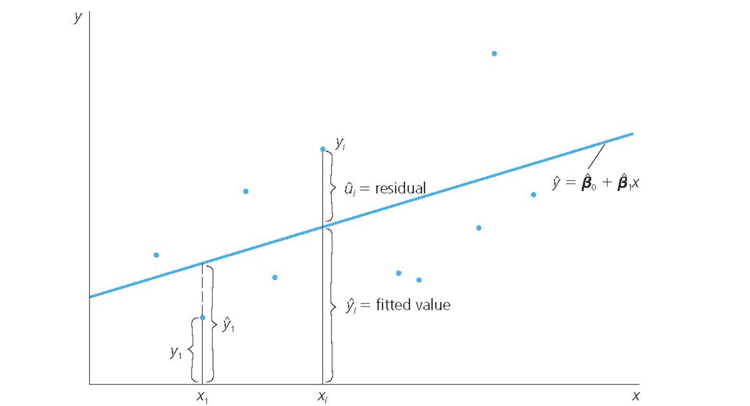
Interpretation of Regression Line: \(\hat{\beta_1}\) amount of change of y when x changes by one unit

Solution for Best Line: minimize Squared Residuals $\( R^2 =& \frac{ \text{Total Sum of Squars}}{\text{Sum of Squared Errors}} \\ TSS =& \sum(y_i - \bar{y})^2 \\ SSE =& \sum(\hat{\epsilon}_i)^2 = \sum(y_i-\hat{y_i})^2 \)$

Units

Example: \(wage = \beta_0 + \beta_1 educ + e\)​​, wage measured in $

Rules:

• \(dependent * c \implies\hat{\beta_1} * c\)

• \(independent * c \implies \hat{\beta_1}/c\)​ and vice versa (not intercept!)

Interpretation of Logs etc.

Model	dependent	independent	interpretation
Level-Level	y	\(x_j\)	\(\Delta \hat{y} = \beta_j \Delta x_j\)
Level-Log	y	\(log(x_j)\)	\(\Delta \hat{y} = \frac{\beta_j}{100} \% \Delta x_j\)
Log-Level	log(y)	\(x_j\)	\(\% \Delta \hat{y} = 100 \beta_j \Delta x_j\)
Log-Log	log(y)	log(x)	\(\% \Delta \hat{y} = \beta_j \% \Delta x_j\)

Expected Values

Assumptions for unbiasedness

1. Linear in parameters (model represents truth)

2. random sample of population

3. Sample variation of x

4. zero conditional mean: \(E(u|x)=0\)

=> OLS = unbiased estimator if

• \(E(OLS) = \theta\): mean of many samples = always the same

• \(E(\hat{\beta}_{0,1}) = \beta_{0,1}\): mean of estimate = truth

Variance of OLS

Assumption 5: \(Var(u|x) = \sigma^2\) (homoskedasticity)

Variance of \(\beta_1\)

• larger error variance => larger Var

• larger variability of x => larger Var

• larger sample => lower Var

Standard Error: \(se(\beta_1) = \frac{ \sigma^2 }{\sqrt{SST_x}}\)